Ditch Excel and Use Julia Data Frames

Manipulating and visualizing pizza sales data using Julia DataFrames.jl and Plots.jl

Erik Engheim

Oct 27, 2020·19 min read

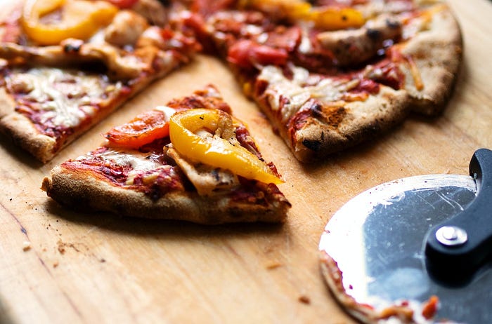
In this story we will look at pizza sales data found here:

https://vincentarelbundock.github.io/Rdatasets/csv/gt/pizzaplace.csv

This kind of data can be manipulated in a spreadsheet application such as Excel and using data frames popular in languages such as R, Python (Pandas) and Julia (DataFrames.jl).

Loading Data

First we will load the data in Julia and pick a subset (id, name, size and price) of columns in the table to work with:

using DataFrames, CSV

url = "https://vincentarelbundock.github.io/Rdatasets/csv/gt/pizzaplace.csv"
filename = download(url)
all_pizzas = CSV.read(filename)

# Get rid of column with row numbers
all_pizzas = all_pizzas[:, 2:end]

# Pick most interesting columns
pz = select(all_pizzas, :id, :name, :size, :price)

We can look at the first view rows to see what this looks like in the Julia REPL (Read Evaluate Program Loop):

julia> first(pz, 4)
4×4 DataFrame
│ Row │ id          │ name        │ size   │ price   │
│     │ String      │ String      │ String │ Float64 │
├─────┼─────────────┼─────────────┼────────┼─────────┤
│ 1   │ 2015-000001 │ hawaiian    │ M      │ 13.25   │
│ 2   │ 2015-000002 │ classic_dlx │ M      │ 16.0    │
│ 3   │ 2015-000002 │ mexicana    │ M      │ 16.0    │
│ 4   │ 2015-000002 │ thai_ckn    │ L      │ 20.75   │

julia> nrow(pz)
49574

However we are currently looking at the first 4 rows. But as you can see there are almost 50 thousand rows in this dataset so not very practical to paste into a spreadsheet. Also for educational reasons, will pick a smaller subset.

Sampling Data

We are going to pick a random sample of 16 rows from the 49 574 rows we have loaded in. To do that we will randomly shuffle the row indices from 1 to 49 574.

julia> using Random

julia> rows = shuffle(1:nrow(pz))

We can then pick the first 16 rows of these shuffled rows to get 16 random rows from our original data:

julia> sample = pz[rows[1:16], :]
16×4 DataFrame
│ Row │ id          │ name         │ size   │ price   │
│     │ String      │ String       │ String │ Float64 │
├─────┼─────────────┼──────────────┼────────┼─────────┤
│ 1   │ 2015-000348 │ thai_ckn     │ S      │ 12.75   │
│ 2   │ 2015-007731 │ green_garden │ S      │ 12.0    │
│ 3   │ 2015-014409 │ hawaiian     │ S      │ 10.5    │
│ 4   │ 2015-017919 │ sicilian     │ S      │ 12.25   │
│ 5   │ 2015-015337 │ prsc_argla   │ M      │ 16.5    │
│ 6   │ 2015-006190 │ ital_veggie  │ S      │ 12.75   │
│ 7   │ 2015-015481 │ spin_pesto   │ S      │ 12.5    │
│ 8   │ 2015-007865 │ hawaiian     │ L      │ 16.5    │
│ 9   │ 2015-001928 │ bbq_ckn      │ L      │ 20.75   │
│ 10  │ 2015-017298 │ cali_ckn     │ S      │ 12.75   │
│ 11  │ 2015-018872 │ four_cheese  │ L      │ 17.95   │
│ 12  │ 2015-018036 │ four_cheese  │ L      │ 17.95   │
│ 13  │ 2015-011238 │ classic_dlx  │ L      │ 20.5    │
│ 14  │ 2015-013366 │ classic_dlx  │ M      │ 16.0    │
│ 15  │ 2015-014380 │ bbq_ckn      │ M      │ 16.75   │
│ 16  │ 2015-020245 │ ital_cpcllo  │ S      │ 12.0    │

You read the syntax used in the square brackets as [rows, columns], where rows is a collection of rows you want. This could be a range, vector or single scalar value. The same applies to columns.

Transfer Pizza Sales to Spreadsheet

However we cannot easily copy and paste data on this “pretty” format into a spreadsheet application such as Excel. We want it on CSV format. Fortunately Julia display system allows us to display the same data in many different formats.

In the Julia REPL, what actually happens automatically is that the display function gets called like this:

julia> display(sample)
16×4 DataFrame
│ Row │ id          │ name         │ size   │ price   │
│     │ String      │ String       │ String │ Float64 │
├─────┼─────────────┼──────────────┼────────┼─────────┤
│ 1   │ 2015-000348 │ thai_ckn     │ S      │ 12.75   │
│ 2   │ 2015-007731 │ green_garden │ S      │ 12.0    │
│ 3   │ 2015-014409 │ hawaiian     │ S      │ 10.5    │
│ 4   │ 2015-017919 │ sicilian     │ S      │ 12.25   │
│ 5   │ 2015-015337 │ prsc_argla   │ M      │ 16.5    │
│ 6   │ 2015-006190 │ ital_veggie  │ S      │ 12.75   │
│ 7   │ 2015-015481 │ spin_pesto   │ S      │ 12.5    │
│ 8   │ 2015-007865 │ hawaiian     │ L      │ 16.5    │
│ 9   │ 2015-001928 │ bbq_ckn      │ L      │ 20.75   │
│ 10  │ 2015-017298 │ cali_ckn     │ S      │ 12.75   │
│ 11  │ 2015-018872 │ four_cheese  │ L      │ 17.95   │
│ 12  │ 2015-018036 │ four_cheese  │ L      │ 17.95   │
│ 13  │ 2015-011238 │ classic_dlx  │ L      │ 20.5    │
│ 14  │ 2015-013366 │ classic_dlx  │ M      │ 16.0    │
│ 15  │ 2015-014380 │ bbq_ckn      │ M      │ 16.75   │
│ 16  │ 2015-020245 │ ital_cpcllo  │ S      │ 12.0    │

However this function can also take a MIME type as an argument, which is used when e.g. Julia is used in a Notebook that supports richer graphical capabilities. In a notebook we supply the text/html MIME type, but in this case we want our data in CSV format:

julia> display("text/csv", sample)
"id","name","size","price"
"2015-000348","thai_ckn","S",12.75
"2015-007731","green_garden","S",12.0
"2015-014409","hawaiian","S",10.5
"2015-017919","sicilian","S",12.25
"2015-015337","prsc_argla","M",16.5
"2015-006190","ital_veggie","S",12.75
"2015-015481","spin_pesto","S",12.5
"2015-007865","hawaiian","L",16.5
"2015-001928","bbq_ckn","L",20.75
"2015-017298","cali_ckn","S",12.75
"2015-018872","four_cheese","L",17.95
"2015-018036","four_cheese","L",17.95
"2015-011238","classic_dlx","L",20.5
"2015-013366","classic_dlx","M",16.0
"2015-014380","bbq_ckn","M",16.75
"2015-020245","ital_cpcllo","S",12.0

You could just copy and paste this into a spreadsheet application. But there are many ways of doing this. We could write to file using the CSV package:

julia> CSV.write("pizza-sales.csv", sample)
"pizza-sales.csv"

But you could achieve this even by leveraging MIME types with show:

julia> open("pizza-sales.csv", "w") do io
           show(io, MIME("text/csv"), sample)
       end

Or what about being a bit crazy, and using an IOBuffer with a clipboard:

julia> buf = IOBuffer();
julia> CSV.write(buf, sample);
julia> clipboard(String(take!(buf)))

After this the pizza sales data will be on the clipboard and you can paste it into your favorite spreadsheet application.

Instead of take! we could have used seekstart to go to the beginning of the IOBuffer and read from it normally. However the benefit of using take! is that you empty the buffer so it no longer consumes any memory to hold the CSV data.

Eventually you get a table as shown below in your preferred spreadsheet application, whether that is Excel, Numbers or Google Sheets. What is useful in a spreadsheet is that you can e.g. click a column and get all sorts of statistics. Notice how we get the sum, average, min and max value.

Getting the same in Julia is easy. We just need to import the Statistics package.

julia> using Statistics

julia> sum(sample.price)
240.39999999999998

julia> mean(sample.price)
15.024999999999999

julia> minimum(sample.price)
10.5

julia> maximum(sample.price)
20.75

julia> nrow(sample)
16

Plotting Histograms

When doing Exploratory Data Analysis (EDA) one of the first useful things you can do to get a sense of the data, is to plot interesting data in histograms.

julia> histogram(sample.price, bins = 4)

We can compare the histogram for the sample data with a similar histogram for the whole dataset:

julia> histogram(pz.price, bins = 6)

We can combine plots and get them side by side. But when comparing plots it is good to have the data in similar ranges. So we will use the xaxis and yaxis attributes to specify the ranges.

julia> p1 = histogram(sample.price,
               bins  = 4,
               xlims = (0, 40),
               xaxis = "price",
               yaxis = "count",
               legend=nothing)
               
julia> p2 = histogram(pz.price,
               bins  = 4,
               xlims = (0, 40),
               xaxis = "price",
               yaxis = "count",
               legend=nothing)
               
julia> p = plot(p1, p2)

If you want to include your plots into reports and documents you can save them to disk using the savefig function. It will pickup desired format to use based on your filename extension. .png, .pdf, .svg and several other formats are supported:

julia> savefig(p, "pizza-price-hist.png")

Interesting Questions to Ask About Our Data

After looking at the data we may develop some questions about the data which we want to have answered, such as:

• What are the most sold pizzas?
• What size of pizza, small, medium, large etc is sold the most?
• What pizza brings in the most revenue?
• How much is typically spent on each pizza order?

A lot of this kind of data cannot be pulled directly out of the data. We will have to group related data. E.g. to find out how much is spent on each order, we would have to group every row belonging to the same order and add up the sales price of every pizza in that order.

To find out which pizza brings in the most revenue, we would have to group rows by pizza name and sum up price for each row.

Thus to be able to answer such questions we need to learn more about how to filter, group and combine data in a DataFrame.

Slicing and Dicing Data Frames

Working with Data Frames we got several key functions that help us manipulate the data:

• select Picks a subset of columns, and possibly rename or transform the values in column.
• transform Similar to select except we are not removing any columns. We are just renaming and transforming selected columns.
• groupby Turns a table into multiple tables. The splitting is done by making a table for each unique value of a particular selected column.
• combine Takes multiple tables and turn them into one table again. Allows you collapse all rows in each table into a single row.
• join Let you match up a column in two different tables to join them into one table.

For anyone who has worked with SQL, many of these operations will be familiar. These functions pick, rename and transform rows using similar syntax.

julia> tiny = first(sample, 3)
3×4 DataFrame
│ Row │ id          │ name         │ size   │ price   │
│     │ String      │ String       │ String │ Float64 │
├─────┼─────────────┼──────────────┼────────┼─────────┤
│ 1   │ 2015-000348 │ thai_ckn     │ S      │ 12.75   │
│ 2   │ 2015-007731 │ green_garden │ S      │ 12.0    │
│ 3   │ 2015-014409 │ hawaiian     │ S      │ 10.5    │

We can pick a specific column and do nothing with it:

julia> select(tiny, :price)
3×1 DataFrame
│ Row │ price   │
│     │ Float64 │
├─────┼─────────┤
│ 1   │ 12.75   │
│ 2   │ 12.0    │
│ 3   │ 10.5    │

julia> transform(tiny, :price)
3×4 DataFrame
│ Row │ id          │ name         │ size   │ price   │
│     │ String      │ String       │ String │ Float64 │
├─────┼─────────────┼──────────────┼────────┼─────────┤
│ 1   │ 2015-000348 │ thai_ckn     │ S      │ 12.75   │
│ 2   │ 2015-007731 │ green_garden │ S      │ 12.0    │
│ 3   │ 2015-014409 │ hawaiian     │ S      │ 10.5    │

For transform this operation is rather pointless, as you get all the same rows as you started with. With a rename it is even more pointless as you simply end up adding a column with the same values as the column you are renaming.

julia> select(tiny, :price => :cost)
3×1 DataFrame
│ Row │ cost    │
│     │ Float64 │
├─────┼─────────┤
│ 1   │ 12.75   │
│ 2   │ 12.0    │
│ 3   │ 10.5    │

julia> transform(tiny, :price => :cost)
3×5 DataFrame
│ Row │ id          │ name         │ size   │ price   │ cost    │
│     │ String      │ String       │ String │ Float64 │ Float64 │
├─────┼─────────────┼──────────────┼────────┼─────────┼─────────┤
│ 1   │ 2015-000348 │ thai_ckn     │ S      │ 12.75   │ 12.75   │
│ 2   │ 2015-007731 │ green_garden │ S      │ 12.0    │ 12.0    │
│ 3   │ 2015-014409 │ hawaiian     │ S      │ 10.5    │ 10.5    │

The benefit becomes more clear when you are performing value transformations using functions.

julia> select(tiny, :price => mean)
3×1 DataFrame
│ Row │ price_mean │
│     │ Float64    │
├─────┼────────────┤
│ 1   │ 11.75      │
│ 2   │ 11.75      │
│ 3   │ 11.75      │

julia> transform(tiny, :price => mean)
3×5 DataFrame
│ Row │ id          │ name         │ size   │ price   │ price_mean │
│     │ String      │ String       │ String │ Float64 │ Float64    │
├─────┼─────────────┼──────────────┼────────┼─────────┼────────────┤
│ 1   │ 2015-000348 │ thai_ckn     │ S      │ 12.75   │ 11.75      │
│ 2   │ 2015-007731 │ green_garden │ S      │ 12.0    │ 11.75      │
│ 3   │ 2015-014409 │ hawaiian     │ S      │ 10.5    │ 11.75      │

However these transformations are pointless as we end up with the same average for every row. The reason is that the functions supplied always take as argument the whole column, and needs to spit out a value/values for the whole column. mean only gives one output value.

If we want to apply a function to every single value we can easily produce such a function with ByRow. Here is a simple example demonstrating how it works:

julia> round(3.4)
3.0

julia> rounder = ByRow(round);

julia> rounder([1.2, 4.8, 8.3])
3-element Array{Float64,1}:
 1.0
 5.0
 8.0

Thus ByRow gives us a simple way of creating functions which can operate on each row:

julia> select(tiny, :price => ByRow(round))
3×1 DataFrame
│ Row │ price_round │
│     │ Float64     │
├─────┼─────────────┤
│ 1   │ 13.0        │
│ 2   │ 12.0        │
│ 3   │ 10.0        │

julia> transform(tiny, :price => ByRow(round))
3×5 DataFrame
│ Row │ id          │ name         │ size   │ price   │ price_round │
│     │ String      │ String       │ String │ Float64 │ Float64     │
├─────┼─────────────┼──────────────┼────────┼─────────┼─────────────┤
│ 1   │ 2015-000348 │ thai_ckn     │ S      │ 12.75   │ 13.0        │
│ 2   │ 2015-007731 │ green_garden │ S      │ 12.0    │ 12.0        │
│ 3   │ 2015-014409 │ hawaiian     │ S      │ 10.5    │ 10.0        │

We can combine value transformation and column renaming:

julia> transform(tiny, :price => ByRow(round) => :rounded)
3×5 DataFrame
│ Row │ id          │ name         │ size   │ price   │ rounded │
│     │ String      │ String       │ String │ Float64 │ Float64 │
├─────┼─────────────┼──────────────┼────────┼─────────┼─────────┤
│ 1   │ 2015-000348 │ thai_ckn     │ S      │ 12.75   │ 13.0    │
│ 2   │ 2015-007731 │ green_garden │ S      │ 12.0    │ 12.0    │
│ 3   │ 2015-014409 │ hawaiian     │ S      │ 10.5    │ 10.0    │

But does this mean that using functions without ByRow is pointless? No, in fact they are very useful when used with combine, because it works similar to select except when every column selected is transformed by a function that takes the whole column and returns a single value, such as mean you will end up with a single row.

julia> combine(tiny, :price => mean)
1×1 DataFrame
│ Row │ price_mean │
│     │ Float64    │
├─────┼────────────┤
│ 1   │ 11.75      │

But if you don’t then combine will basically have the same behavior as select:

julia> combine(tiny, :name, :price => mean)
3×2 DataFrame
│ Row │ name         │ price_mean │
│     │ String       │ Float64    │
├─────┼──────────────┼────────────┤
│ 1   │ thai_ckn     │ 11.75      │
│ 2   │ green_garden │ 11.75      │
│ 3   │ hawaiian     │ 11.75      │

Splitting and Recombining Tables

The real power of combine however comes from splitting a data frame up into groups with groupby and then recombining these again to a table.

The trick is to use use these with functions that take multiple elements in and produce a single output such as:

• length Count number of elements. E.g. how many medium medium pizzas are there.
• sum Add up values in column.
• mean Find the arithmetic mean (average).

Let us use this to figure out how many pizzas there are of each size:

julia> sizes = groupby(sample, :size)
GroupedDataFrame with 3 groups based on key: size
Group 1 (7 rows): size = "M"
│ Row │ id          │ name         │ size   │ price   │
│     │ String      │ String       │ String │ Float64 │
├─────┼─────────────┼──────────────┼────────┼─────────┤
│ 1   │ 2015-018649 │ pepperoni    │ M      │ 12.5    │
│ 2   │ 2015-011258 │ hawaiian     │ M      │ 13.25   │
│ 3   │ 2015-009299 │ veggie_veg   │ M      │ 16.0    │
│ 4   │ 2015-010260 │ peppr_salami │ M      │ 16.5    │
│ 5   │ 2015-017124 │ hawaiian     │ M      │ 13.25   │
│ 6   │ 2015-011800 │ thai_ckn     │ M      │ 16.75   │
│ 7   │ 2015-008107 │ ckn_alfredo  │ M      │ 16.75   │
Group 2 (5 rows): size = "L"
│ Row │ id          │ name        │ size   │ price   │
│     │ String      │ String      │ String │ Float64 │
├─────┼─────────────┼─────────────┼────────┼─────────┤
│ 1   │ 2015-000629 │ spin_pesto  │ L      │ 20.75   │
│ 2   │ 2015-011532 │ spinach_fet │ L      │ 20.25   │
│ 3   │ 2015-019947 │ pepperoni   │ L      │ 15.25   │
│ 4   │ 2015-002630 │ thai_ckn    │ L      │ 20.75   │
│ 5   │ 2015-018629 │ cali_ckn    │ L      │ 20.75   │
Group 3 (4 rows): size = "S"
│ Row │ id          │ name         │ size   │ price   │
│     │ String      │ String       │ String │ Float64 │
├─────┼─────────────┼──────────────┼────────┼─────────┤
│ 1   │ 2015-017814 │ green_garden │ S      │ 12.0    │
│ 2   │ 2015-012022 │ veggie_veg   │ S      │ 12.0    │
│ 3   │ 2015-010260 │ southw_ckn   │ S      │ 12.75   │
│ 4   │ 2015-010846 │ big_meat     │ S      │ 12.0    │

sizes is not a collection of groups represented by the GroupedDataFrame type. We can recombine these groups:

julia> combine(sizes, :size => length)
3×2 DataFrame
│ Row │ size   │ size_length │
│     │ String │ Int64       │
├─────┼────────┼─────────────┤
│ 1   │ M      │ 7           │
│ 2   │ L      │ 5           │
│ 3   │ S      │ 4           │

We could rename column for a nicer table:

julia> combine(sizes, :size => length => :amount)
3×2 DataFrame
│ Row │ size   │ amount │
│     │ String │ Int64  │
├─────┼────────┼────────┤
│ 1   │ M      │ 7      │
│ 2   │ L      │ 5      │
│ 3   │ S      │ 4      │

We can use this for the whole dataset and plot a histogram:

julia> pz_sizes = combine(groupby(pz, :size), :size => length => :amount)

julia> bar(pz_sizes.size, pz_sizes.amount, bins=5, legend=nothing)

One problem with this plot that you can see is that the sizes are not sorted in order S, M, L, XL, XXL which makes it confusing. How can we solve that?

Joining Tables

There are a lot of ways of defining an order for pizza sizes, but here I will solves this by joining tables, because it is something you should know how to do anyway. A simple solution is to give sizes a numerical value.

The standard diameters of pizzas are:

• Small — 26 cm
• Medium — 31 cm
• Large — 36 cm
• X-Large — 41 cm
• Jumbo — 46 cm

We will use Jumbo size for XXL. Let us Make a table that maps pizza sizes to diameters:

julia> diameters = DataFrame(size = ["S", "M", "L", "XL", "XXL"],
                             diameter = [26, 31, 36, 41, 46])
5×2 DataFrame
│ Row │ size   │ diameter │
│     │ String │ Int64    │
├─────┼────────┼──────────┤
│ 1   │ S      │ 26       │
│ 2   │ M      │ 31       │
│ 3   │ L      │ 36       │
│ 4   │ XL     │ 41       │
│ 5   │ XXL    │ 46       │

To join we need to specify which column will be the primary key, or the value we will join on. That will be size since that is the only column that exists in both tables:

julia> pz = join(pz, diameters, on=:size);

julia> select(pz, :name, :size, :diameter, :price)
49574×4 DataFrame
│ Row   │ name         │ size   │ diameter │ price   │
│       │ String       │ String │ Int64    │ Float64 │
├───────┼──────────────┼────────┼──────────┼─────────┤
│ 1     │ spin_pesto   │ L      │ 36       │ 20.75   │
│ 2     │ pepperoni    │ M      │ 31       │ 12.5    │
│ 3     │ hawaiian     │ M      │ 31       │ 13.25   │
│ 4     │ spinach_fet  │ L      │ 36       │ 20.25   │
│ 5     │ veggie_veg   │ M      │ 31       │ 16.0    │

But let us get back to our original task. We want to insert diameters into table over how many of the pizzas sold are of a particular type:

julia> pz_sizes = combine(groupby(pz, :size), :size => length => :amount)

julia> pz_sizes = join(pz_sizes, diameters, on=:size)
5×3 DataFrame
│ Row │ size   │ amount │ diameter │
│     │ String │ Int64  │ Int64    │
├─────┼────────┼────────┼──────────┤
│ 1   │ M      │ 15635  │ 31       │
│ 2   │ L      │ 18956  │ 36       │
│ 3   │ S      │ 14403  │ 26       │
│ 4   │ XL     │ 552    │ 41       │
│ 5   │ XXL    │ 28     │ 46       │

And let us sort by diameter:

julia> sort!(pz_sizes, :diameter)
5×3 DataFrame
│ Row │ size   │ amount │ diameter │
│     │ String │ Int64  │ Int64    │
├─────┼────────┼────────┼──────────┤
│ 1   │ S      │ 14403  │ 26       │
│ 2   │ M      │ 15635  │ 31       │
│ 3   │ L      │ 18956  │ 36       │
│ 4   │ XL     │ 552    │ 41       │
│ 5   │ XXL    │ 28     │ 46       │

Now we got something better suited for plotting in a bar plot.

bar(pz_sizes.size, pz_sizes.amount, bins=5, legend=nothing)

Plotting is of course an art. To get a sense of what dominates ones sales it may make more sense to use a pie chart:

pie(pz_sizes.size, pz_sizes.amount, title="Most sold pizza sizes")

What pizza size is most popular?

Looking at our charts we can see that most pizzas sold is the large one with medium on a solid second. But how does it look in terms of pizza slices eaten?

Basically what we want to know is what kind of pizza is consumed most. Since we know the diameter, we can calculate the area of each pizza.

julia> area(r) = π*r^2
julia> pz_sizes.area = area.(pz_sizes.diameter ./ 2);

To make it a bit nicer to display I will just round off the calculated areas:

julia> pz_sizes.area = round.(Int, pz_sizes.area)
julia> pz_sizes
5×4 DataFrame
│ Row │ size   │ amount │ diameter │ area  │
│     │ String │ Int64  │ Int64    │ Int64 │
├─────┼────────┼────────┼──────────┼───────┤
│ 1   │ S      │ 14403  │ 26       │ 531   │
│ 2   │ M      │ 15635  │ 31       │ 755   │
│ 3   │ L      │ 18956  │ 36       │ 1018  │
│ 4   │ XL     │ 552    │ 41       │ 1320  │
│ 5   │ XXL    │ 28     │ 46       │ 1662  │

Now we can calculate the total area for each pizza type:

julia> pzs = pz_sizes
julia> pzs.total_area = pzs.area .* pzs.amount
julia> pzs
5×5 DataFrame
│ Row │ size   │ amount │ diameter │ area  │ total_area │
│     │ String │ Int64  │ Int64    │ Int64 │ Int64      │
├─────┼────────┼────────┼──────────┼───────┼────────────┤
│ 1   │ S      │ 14403  │ 26       │ 531   │ 7647993    │
│ 2   │ M      │ 15635  │ 31       │ 755   │ 11804425   │
│ 3   │ L      │ 18956  │ 36       │ 1018  │ 19297208   │
│ 4   │ XL     │ 552    │ 41       │ 1320  │ 728640     │
│ 5   │ XXL    │ 28     │ 46       │ 1662  │ 46536      │

And let us make it more interesting by plotting how many pizzas have been bought and compare it to the area of pizza consumed of each type:

p1 = pie(pzs.size, pzs.amount, title="Pizzas by Numbers");
p2 = pie(pzs.size, pzs.total_area, title="Pizzas by Area");
p  = plot(p1, p2)

What pizza brings in the most revenue?

We begin by creating a subgroup for each pizza.

groupby(pz, :name)

We can then add up the price of each pizza sold with the same name.

combine(groupby(pz, :name), :price => sum => :revenue)

But we want this sorted so we can find the top 10 most sold pizzas.

julia> pizzas = groupby(pz, :name);
julia> pizzas = combine(pizzas, :price => sum => :revenue);

julia> top10 = first(sort(pizzas, :revenue, rev=true), 10)
10×2 DataFrame
│ Row │ name        │ revenue │
│     │ String      │ Float64 │
├─────┼─────────────┼─────────┤
│ 1   │ thai_ckn    │ 43434.2 │
│ 2   │ bbq_ckn     │ 42768.0 │
│ 3   │ cali_ckn    │ 41409.5 │
│ 4   │ classic_dlx │ 38180.5 │
│ 5   │ spicy_ital  │ 34831.2 │
│ 6   │ southw_ckn  │ 34705.8 │
│ 7   │ ital_supr   │ 33476.8 │
│ 8   │ hawaiian    │ 32273.2 │
│ 9   │ four_cheese │ 32265.7 │
│ 10  │ sicilian    │ 30940.5 │

We can can visualize this with a bar chart:

bar(top10.name, top10.revenue, label="pizza revenue")

How much is typically spent on each pizza order?

To get how much is spent on each pizza order we create a subgroup of the data frame for each unique order id:

julia> groupby(pz, :id)
GroupedDataFrame with 21350 groups based on key: id
First Group (1 row): id = "2015-000001"
│ Row │ id          │ name     │ size   │ price   │ diameter │ area    │
│     │ String      │ String   │ String │ Float64 │ Float64  │ Float64 │
├─────┼─────────────┼──────────┼────────┼─────────┼──────────┼─────────┤
│ 1   │ 2015-000001 │ hawaiian │ M      │ 13.25   │ 0.31     │ 0.0755  │
⋮
Last Group (1 row): id = "2015-021350"
│ Row │ id          │ name    │ size   │ price   │ diameter │ area    │
│     │ String      │ String  │ String │ Float64 │ Float64  │ Float64 │
├─────┼─────────────┼─────────┼────────┼─────────┼──────────┼─────────┤
│ 1   │ 2015-021350 │ bbq_ckn │ S      │ 12.75   │ 0.26     │ 0.0531  │

We can then recombine these groups by summing up the price column, which allows us to collapse each sub-group into a single row in a new table. In this table, there is just one line for each order:

julia> orders = combine(groupby(pz, :id), :price => sum => :sum)
21350×2 DataFrame
│ Row   │ id          │ sum     │
│       │ String      │ Float64 │
├───────┼─────────────┼─────────┤
│ 1     │ 2015-000001 │ 13.25   │
│ 2     │ 2015-000002 │ 92.0    │
│ 3     │ 2015-000003 │ 37.25   │
│ 4     │ 2015-000004 │ 16.5    │

Let us do some simple exploration of this data first. It is always a good thing to look at minimums, maximums, mean and median value.

julia> minimum(orders.sum)
9.75

julia> maximum(orders.sum)
444.2

julia> mean(orders.sum)
38.30726229508197

julia> median(orders.sum)
32.5

There is a shorthand for getting all of this data in one swoop:

julia> describe(orders, :min, :max, :mean, :median)
2×5 DataFrame
│ Row │ variable │ min         │ max         │ mean    │ median │
│     │ Symbol   │ Any         │ Any         │ Union…  │ Union… │
├─────┼──────────┼─────────────┼─────────────┼─────────┼────────┤
│ 1   │ id       │ 2015-000001 │ 2015-021350 │         │        │
│ 2   │ sum      │ 9.75        │ 444.2       │ 38.3073 │ 32.5   │

We can confirm this initial impression by plotting the histogram showing us the value distribution. We can see the bulk of the orders are below 50 dollars.

julia> histogram(
           orders.sum,
           xaxis="order sum",
           yaxis="frequency",
           xticks=0:50:400,
           legend=nothing)

Now you may wonder, how do I know all the settings which can be used to get the plots right? Part of this is really gradual experimentation. Tweaking setting repeatedly until you get a desired plot.

Final Words

We have just scratched the surface of what is possible with Julia’s data frames and plotting libraries, but hopefully this gave you a flavor.

You can look at a slightly different treatment of the same Pizza data using a different plotting library Gadfly, in the previous story on plotting that I wrote. Other resources:

• Using various other Julia plotting libraries. E.g. covers VegaLite, which has cool pie charts.
• Plots.jl reference card. I advice just printing out this overview page.